Risk Limiting Audits
Why RLAs?
Risk Limiting Audits (RLAs) can provide an additional safeguard for election results, giving you the confidence that election results are accurate.
It is worth noting that even without RLAs, there is already strong basis for voters to trust that other voters will verify their vote using the Verification #. Once an election outcome does not go their preferred way, supporters of the losing candidate have a strong incentive to verify that their vote was tallied correctly using their Verification #. SIV automatically stores all necessary verification materials on voters' device, so that they can still easily check their vote at any time without any prior preparation. If anything did go wrong, they have all the evidence needed to fully prove that their vote was not cast correctly.
However, using Risk Limiting Audits, we can achieve an even higher level of assurance of correct results.
Carrying Out a SIV RLA
Conducting a SIV Risk Limiting Audit involves selecting a random sample of votes and verifying their accuracy.
An election official and/or civil organizations should contact the selected voters through an appropriate channel, such as a phone-call and/or email. The voter will be asked to self-verify the accuracy of their vote using the necessary tools, such as a verification number and, if desired, a second device check. The voter will be guided through the process and upon completion, should inform the official of the outcome without disclosing their specific vote. A statement confirming that there are or are not any discrepancies would be sufficient.
It is important to ensure that the protocol adopted for a SIV RLA does not compromise the privacy of the individual voters' selections. Therefore, the election official must not ask about the specifics of the voter's choice, and the voter must not be asked to show evidence or disclose who they voted for.
Carrying out a Risk Limiting Audit can be vastly more efficient when combined with Anti-Malware Codes. This is because using Anti-Malware Codes is an asynchronous process: all randomly sampled voters can perform it in parallel, rather than auditors needing to walk each voter through their confirmation one at a time.
People carrying out an RLA may also want to collect cryptographic signatures from voters that prove their device participated in the election, to prevent the RLA itself from being vulnerable to fraud.
RLA Calculator
You can adjust these numbers to see how different Margins of Victory, Samples Sizes, and # of Compromised Votes found all affect the implied statistical confidence.
The underlying mathematics is explained below.
The Math Behind RLAs
Let's examine a concrete example. Imagine you participate in an election where you had the chance to cast your vote for one of two candidates: George Washington or Abraham Lincoln. You vote for Abraham Lincoln. But the final results show George Washington received 10 votes and Abraham Lincoln only 5.
Because your preferred candidate lost, you feel strongly motivated to confirm that the election results are accurate. What do you need to do to gain strong confidence?
You start by checking that the list of anonymized votes indeed adds up to 10 for Washington and 5 for Lincoln. Then you check that your own Verification # is in the list of anonymized votes, with your correct selection alongside it, and confirm your own device wasn't manipulated by malware. This tells you that at least 1 out of the 15 total votes is correct, but what about the other 14?
An Unoptimized Process
Do all of them need to be checked, or how many confirmations are needed to gain full confidence in the outcome?
- If the outcome was 10-to-5, that means the "Margin of Victory" was 5 votes (10 minus 5).
- So if any 3 of the 10 Washington votes had been flipped from originally-Lincoln, the "true count" would have been 8 Lincoln to 7 Washington, changing the winner.
- Thus, the Margin of Error is that 2 votes could have been flipped, without changing the final winner.
- Therefore, you could be fully sure that the "true winner" won after confirmation from at least 13 voters (15 minus 2), who would confirm that they checked their vote was counted correctly, all without needing to compromise their privacy to know how they voted.
This is a sort of "naive (opens in a new tab)", unoptimized solution.
Optimizing With Statistical Sampling Math
Rather than needing to confirm 13 out of 15 votes, if we use random statistical sampling, we can gain quite high confidence in the outcome, far more efficiently.
Important note: "Random sampling" does not mean "ask whoever is closest at hand", but specifically to use a random number generator (opens in a new tab) to identify a random voter to check.
Continuing with our 10 Washington to 5 Lincoln example...
- Our Margin of Error remains 2, so at least 3 votes must have been flipped to change the final winner.
(winners_votes - runner_ups_votes) / 2 - Let us randomly sample just 1 out of the 15 voters, and confirm with the voter that their vote was included correctly in the final tally, without needing to learn how they voted.
- If the election was fraudulent, at least 3 of the votes must have been flipped, & 12 could remain as originally cast. So testing this first voter to confirm their vote was correct should "detect" if the election was fraudulent with probability 3 out of 15, or 20% of the time. In other words, just this single test can bring our confidence in a "correct" winner from 0% to 20%.
- If we then randomly sample another voter, and they confirm their vote was counted correctly, this could have detected a cheating election with probability 3 out of 14: each test decreases the denominator by one.
- The highest possible chance that our first sample did not catch present cheating was 80%, and the chance that the second sample alone did not is 11/14, or ~78.6%. But the chance that neither of them together did is
(12/15) * (11/14), or ~62.9%. So our overall confidence in correct results goes from 0% before any samples, to 20% after just 1 sample, to 37.1% after 2 samples. - A third sample can detect 3 out of the 13 remaining votes, and might fail to catch 10/13 times. So after three samples, the total "false positive" rate becomes
(12/15) * (11/14) * (10/13), or ~48.4%. So with just 3 samples, we've already gained over 51% confidence that the "correct" winner won.
Here is the basic formula continued for all 15 votes:
| this round | total | |||||
|---|---|---|---|---|---|---|
| votes checked | possible frauds | # votes | chance of catching fraud | uncaught from this check | total uncaught chance | total confidence |
| 1 | 3 | 15 | 20% | 80% | 80% | 20.0% |
| 2 | 3 | 14 | 21.4% | 78.6% | 62.9% | 37.1% |
| 3 | 3 | 13 | 23% | 76.9% | 48.4% | 51.6% |
| 4 | 3 | 12 | 25% | 75.0% | 36.3% | 63.7% |
| 5 | 3 | 11 | 27% | 72.7% | 26.4% | 73.6% |
| 6 | 3 | 10 | 30% | 70.0% | 18.5% | 81.5% |
| 7 | 3 | 9 | 33% | 66.7% | 12.3% | 87.7% |
| 8 | 3 | 8 | 38% | 62.5% | 7.7% | 92.3% |
| 9 | 3 | 7 | 43% | 57.1% | 4.4% | 95.6% |
| 10 | 3 | 6 | 50% | 50% | 2.2% | 97.8% |
| 11 | 3 | 5 | 60% | 40% | 0.9% | 99.1% |
| 12 | 3 | 4 | 75% | 25% | 0.2% | 99.8% |
| 13 | 3 | 3 | 100% | 0% | 0.0% | 100.0% |
| 14 | 3 | 2 | 100% | 0% | 0.0% | 100.0% |
| 15 | 3 | 1 | 100% | 0% | 0.0% | 100.0% |
The power of a Risk Limiting Audit (RLA) is that you don't need to check all 15 votes. This RLA math shows that in this sample 15-vote election, just 3 random checks alone gives over 51% confidence, 6 checks gives over 81% confidence, and 8 checks give over 92% confidence.
Note that "confidence" is shorthand for "If there had been enough compromised votes to flip the election's winner, we've now manually reconfirmed enough votes that we would have detected it this % of this time".
Deriving A General Formula
First, we'll note the specific closed form equation to make calculations much easier. Given an election's total_votes_cast & margin_of_error (difference between winner's votes & runner up's votes, divided by two), what % confidence is gained from confirming X randomly-sampled votes?
In the case of two votes checked in a 15 vote election with an error margin of 3, the "false positive" formula was (12/15) * (11/14). This can be rewritten as (12*11) / (15*14), or using nCr format (opens in a new tab) as .
This can be generalized for any election as:
false_positive_rate = nChooseR(total_votes - margin_of_error, num_checked) / nChooseR(total_votes, num_checked)
The confidence % is 1 - false_positive rate.
A Larger Example: The 2020 US Presidential Election in Georgia
Now that we have looked at how the math can work for this small 15 vote election, how does it scale for much larger elections?
The 2020 US Presidential Election in Georgia was remarkable for its razor-thin margin. The certified final count (opens in a new tab) was:
| # | % | |
|---|---|---|
| Total Votes Cast | 4,999,958 | 100% |
| Votes for Joe Biden | 2,473,633 | 49.47% |
| Votes for Donald Trump | 2,461,854 | 49.24% |
| Difference | 11,779 | |
| Margin of Error | 5,889 | 0.12% |
The margin of error was only 0.12%, meaning that only about 1 out of every 1000 votes would need to be compromised for a different winner.
Traditional paper elections do not offer voters a way to confirm that their individual vote was accurately counted. Although a different type of Risk-Limiting Audit, known as "Batch Comparison" RLAs, is encouraged and frequently used, it does not verify that the correct votes were counted in the first place ("Ballot-Level Comparison"). Instead, it confirms that the physical vote-tallying equipment worked properly. However, in the 2020 Georgia Election, the margin was too narrow to employ this type of RLA effectively. As a result, all 5 million ballots were manually recounted by hand across all 159 counties over a 10-day period. This constituted the largest hand count of ballots in United States history.
If individual ballots had been verifiable, as SIV allows, we can apply the closed form Risk Limiting Audit math above to calculate the following confidence gained:
| # Checked | % of total Checked | Confidence % Gained |
|---|---|---|
| 1 | 0.00% | 0.12% |
| 10 | 0.00% | 1.17% |
| 100 | 0.00% | 11.12% |
| 1000 | 0.02% | 69.23% |
| 5000 | 0.10% | 99.72% |
| 7500 | 0.15% | 99.986% |
| 10000 | 0.20% | 99.9992% |
Code to re-calculate this table yourself (opens in a new tab)
As shown above, despite the razor thin margin, confirming only 5,000 randomly sampled votes out of the 4,999,958 total cast (about 1 in 1000) can provide 99.72% confidence that the final winner was correct. Doubling the amount checked to 10,000 out of the approximately 5,000,000 total votes results in 99.9992% confidence in correct outcomes.
This means that despite razor-thin margins, this form of individual ballot sampling can achieve very high confidence with high efficiency.
Handling Non-Confirmatory Cases
So far, we have only examined the implied statistical probability when an audit comes back 100% confirmatory. But when checking individual votes, there are three possible scenarios:
- Voter successfully confirms vote was correctly tallied
- Confirmation is inconclusive (e.g. voter can't be reached, refuses to cooperate, or necessary key material was lost)
- Voter discovers the vote is incorrectly tallied (e.g. due to malware, compromised election server, voter credentials stolen such as by a housemate, etc.)
We have covered the confirmatory case (#1) above.
Inconclusive confirmations (#2) are context specific. For example:
- If testing against ballot stuffing, not being able to reach a voter could be treated as a negative result.
- If testing against on-device malware, a voter refusing to cooperate doesn't indicate much positive nor negative about malware. The statistical implication is as if that vote was not checked.
- If testing against on-device malware, vote data mysteriously missing — without a justifiable explanation, such as a physically lost device — could be treated as a negative result.
The discovery of an incorrectly tallied vote (#3) does negatively affect the overall confidence.
Note that if a vote is discovered to have been compromised, the standard SIV protocol for Remediating Compromised Votes can always be used, so voters can submit their correct replacement selections.
But how do these discoveries affect the implied confidence in an election's overall accuracy?
Employing a Binomial Distribution
A Binomial Distribution (opens in a new tab) is a standard statistical tool to model the number of successes in a fixed number of independent trials, where each trial has only two possible outcomes (success or failure), and the probability of success is independent between trials. For example, if you flip a fair coin 10 times, the number of heads you get could be modeled by a binomial distribution with n=10 and p=0.5.
1. The Probability Mass Function (PMF) of a binomial distribution gives the probability of getting exactly successes in independent trials, where each trial has a probability of success.
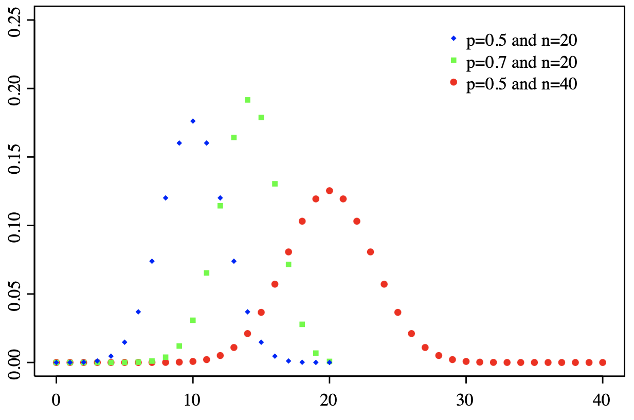
This can be calculated as:
where is the number of trials, is the number of successes, is the probability of success in each trial, and is the binomial coefficient, which is equal to .
This formula can be used to say something like: "If I flipped a coin 20 times, and I saw 10 heads, what is the % chance that if I flipped it another 20 times, I would see exactly heads."
2. The Cumulative Distribution Function (CDF) of a binomial distribution gives the probability of getting no more than successes in independent trials. In other words, this is the sum of adding up each of the successive PMFs.
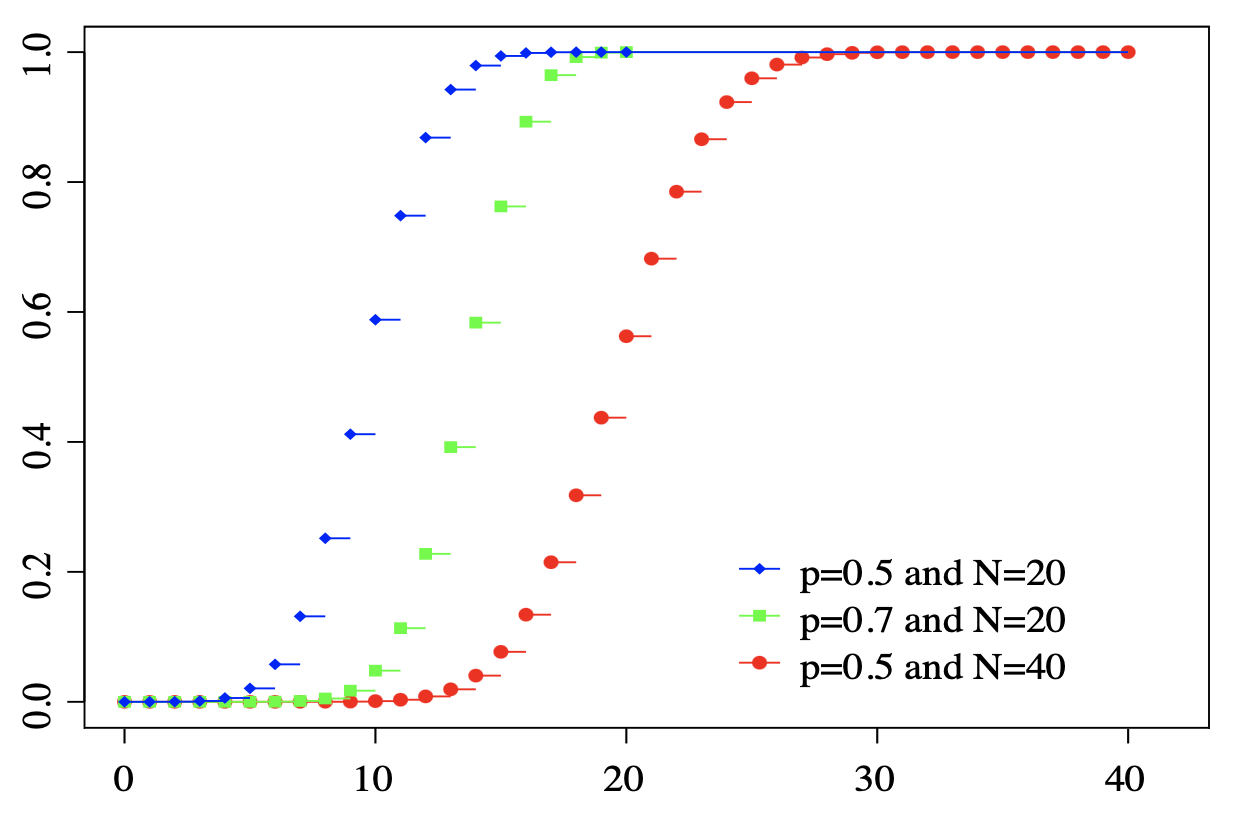
This can be calculated as:
where is the Probability Mass Function given above.
In Post-Election Risk Limiting Audits, we have:
- A Margin of Victory =
- and Margin of Error , rounded up
This Margin of Error is the minimum number of compromised votes to change the winner.
In order for the election results to be accurate, the overall % of compromised votes must be no higher than:
By examining random samples of votes, and recording the rate of successful confirmations vs discovered compromises, we establish statistical trends about the overall set, until we have achieved at least % statistical confidence in the correct winner.
We can use the Cumulative Distribution Function to calculate any implied Confidence in correct results. For our use-case, we will use and to track failures, rather than successes (i.e. the complementary probabilities), which can be done by plugging in:
- k = Margin of Error rate per Sample size
- n = Samples taken
- p = rate of Compromises discovered in the Samples taken
If we were to sample 1000 votes, discovering 2 compromised votes and 998 confirmed ones, the implied PMF would look like:
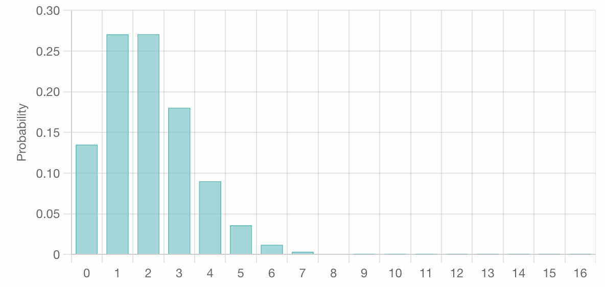
And the CDF would look like:
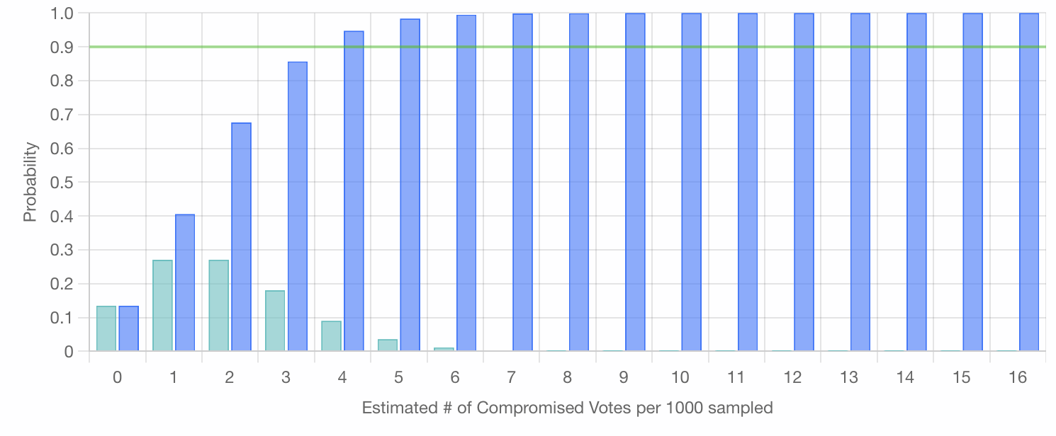
Note that the blue cumulative bar marked 4 (representing the probability that 4 or less compromised votes are present in each successive set of 1000 samples) has crossed the 90% threshold.
That is to say, if this hypothetical election had a Margin of Error of at least 4 votes per 1000 (0.4%), for a Margin of Victory of just 0.8%, discovering only 2 compromised votes in the initial 1000 sampled implies over 90% confidence that the whole election has less than 0.4% compromised, and thus "the correct winner won". Specifically, this implies ~94.8%.
We can extend this approach one step farther and calculate the various minimum Sample Sizes needed to achieve a particular % Confidence level, given different #s of Compromised votes discovered.
To illustrate, we will apply this approach to the 2020 U.S. Presidential Election in Georgia, with its razor-thin Margin of Error of only 0.12%:
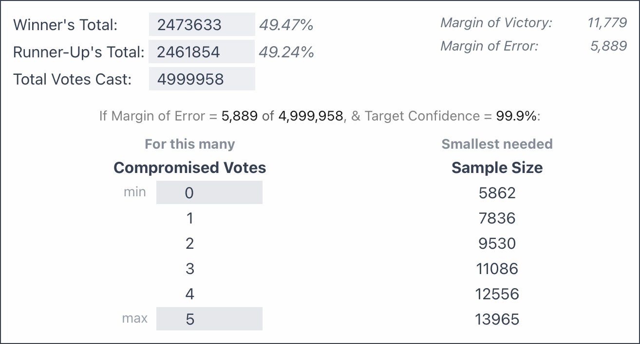
We see similar results as calculated using the initial approach above, where we saw that 5000 confirmations resulted in ~99.7% confidence, just shy of the 5862 needed to cross the 99.9% threshold. But now, by using a Binomial Distribution, we can also factor in the discovery of compromised votes.
In this way, we can achieve very high statistical confidence in elections' accuracy (> 99.9%), despite razor thin margins (0.2%), while only needing to sample a tiny fraction of votes.
All of these statistical tools can be easily applied to any election by using the interactive RLA Calculator at the top of this page.